Quarto Live

Installation

Quarto Live is a Quarto extension that allows you to create interactive documents, including interactive code chunks for many programming language that support WebAssembly, like Python and R. To use Quarto Live, you need to install the extension in your Quarto project. You can do this using the terminal.

If you are working in RStudio, you can quickly get to the terminal for installation by clicking on the tab next to the Console:

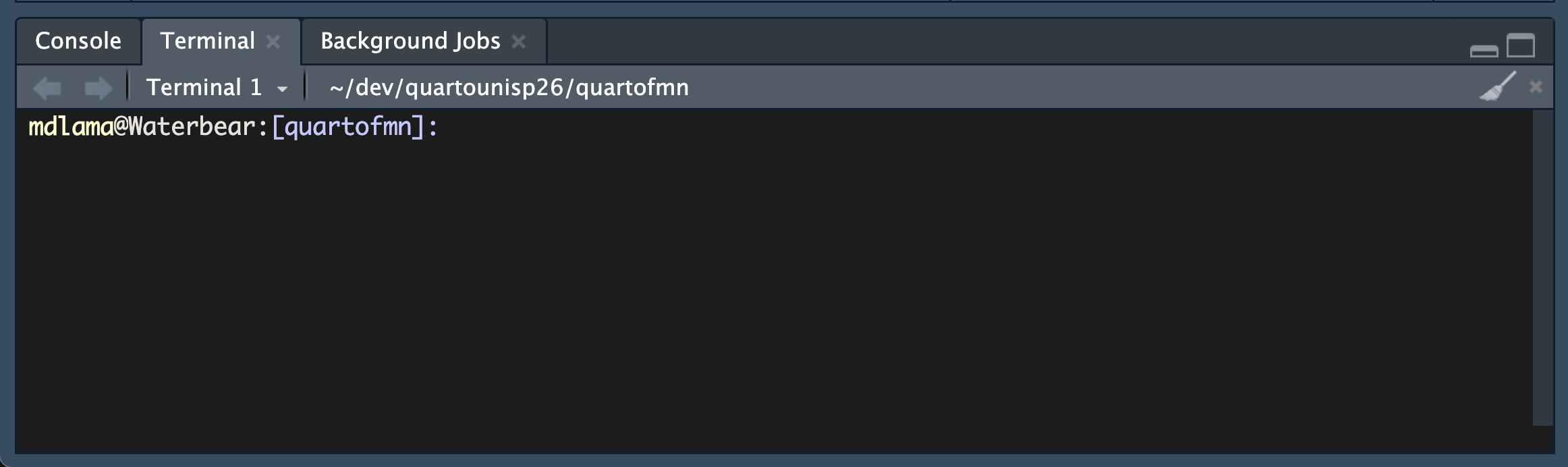
The terminal is located in the tab to the right of the Console.

Once there, you can install the quarto-live package using the following command:

quarto add r-wasm/quarto-live

Getting started

Getting Started Documentation

Helpful Tidbits

Code persistence

One useful feature of Quarto Live is that it allows you to persist code across sessions. This means that if you write some code in a code block and then refresh the page, the code will still be there. This is particularly useful for students that need to step a way from a module and continue work later.

To achieve this, Quarto Live uses the browser’s local storage to save the code in each code block. This means that the code is saved on the user’s device and will persist even if they close the browser or shut down their computer.

Persistence can be set on a block-by-block basis by adding #| persist: true to a block’s YAML. It can also be activated for the entire document by including the following in the YAML header:

---
format: 
  live-html:
    webr:
      cell-options:
        persist: true
---

Execution time limits

Execution time limits can be set for a code block. This can be useful to prevent infinite loops or long-running code from crashing the browser. To set an execution time limit, you can add #| timelimit: <time in seconds> to the code block’s YAML. For example, #| timelimit: 5 would set a time limit of 5 seconds for that code block. Set the time limit to 0 to disable it.

Loading packages and data

Since live HTML documents utilizing WebR run in the browser and not on a server, authors need to be explicit to Quarto Live about which packages and resources to load and make available to the user. This is done using the webr options in the YAML header.

Packages

For example, to load packages, you can include the following in the YAML header:

---
format: live-html
webr:
  packages:
    - ggplot2
    - dplyr
---

---
format: live-html
pyodide:
  packages:
    - matplotlib
    - numpy
    - seaborn
---

Check out the Loading Packages Documentation for more information, including how to load from custom repositories.

Using both R and WebR code blocks

If you are combining R code blocks with WebR code blocks (or Python with pyodide), you will need to load packages in both places, as they run in separate environments. The R code blocks will not have access to packages loaded in WebR code blocks, and vice versa (similar for Python).

Package availability in WebR

Make sure to check if an existing package is available in WebR before trying to load it, as not all R packages are currently supported. You can check the list of available packages. If this link takes too long to load, you can also use this searchable repository created by Bob Rudis.

Files and data

From Quarto’s website:

Normally webr and pyodide code blocks are executed in the reader’s web browser, and so resources local to your own machine are not available for use inside the WebAssembly environment. Instead, there is a Virtual Filesystem (VFS) made available that contains only the minimum required to run R or Python code.

To make additional resources available, you can use the resources option in the YAML header to specify files to be loaded into the VFS. This can include data files, images, or any other resources that your code blocks need to access. For example, if you have a data directory in your Quarto project with multiple datasets, you can include the following in the YAML header to make the entire directory available in the VFS:

---
format: live-html
resources:
  - data
---

Then, you can access the files in the data directory from your code blocks using the path data/filename. For example, if you have a file called mydata.csv in the data directory, you can read it into a WebR code block like this:

```{webr}
mydata <- read.csv("data/mydata.csv")
```

```{pyodide}
import pandas as pd
mydata = pd.read_csv("data/mydata.csv")
```

You can find more information about this feature in the Loading Resources Documentation

Using both R and WebR code blocks

Just like with loading packages, if you are combining R code blocks with WebR code blocks, you will need to load data in both places, as they run in separate environments. The R code blocks will not have access to data loaded in WebR code blocks, and vice versa.

Grading with {gradethis}

Grading with gradethis

Shared environments across code blocks

See the Managing environments documentation.

Prettifying interactive exercises

Default aesthetics

Plot a rectangle using geom_tile centered at (x,y) = (4, 7). Do not specify any other aesthetics.

Hint 2

1ggplot() +
2  geom_tile(mapping = aes(___))

1: Add the geom_tile geom and specify the aesthetics by using the aes() function and assigning it to the mapping argument of geom_tile.
2: Specify the x and y aesthetics as arguments to the aes() function, assigning them their appropriate values.

Solution

1ggplot() +
2  geom_tile(mapping = aes(x = 4, y = 7))

1: Add the geom_tile geom and specify the aesthetics by using the aes() function and assigning it to the mapping argument of geom_tile.
2: Specify the x and y aesthetics as arguments to the aes() function, assigning them their appropriate values.

Markdown

::: {.callout-tip title="Default aesthetics"}
*Plot a rectangle using* `geom_tile` *centered at (x,y) = (4, 7). Do not specify any other aesthetics.*


```{webr}
#| exercise: one-tile-ex-1
#| autorun: FALSE

```

::: { .hint exercise="one-tile-ex-1"}
::: { .callout-note collapse="false"}
## Hint 1

```{r}
ggplot() +       #<1>
  geom_tile(___) #<2>
```
1. Add the `geom_tile` geom and specify the aesthetics by using the `aes()` function and assigning it to the `mapping` argument of `geom_tile`.

:::
:::

::: { .hint exercise="one-tile-ex-1"}
::: { .callout-note collapse="false"}
## Hint 2

```{r}
ggplot() + #<1>
  geom_tile(mapping = aes(___)) #<2>
```
1. Add the `geom_tile` geom and specify the aesthetics by using the `aes()` function and assigning it to the `mapping` argument of `geom_tile`.
2. Specify the x and y aesthetics as arguments to the `aes()` function, assigning them their appropriate values.
:::
:::

::: { .solution exercise="one-tile-ex-1"}
::: { .callout-tip collapse="false"}

## Solution

```{webr}
#| exercise: one-tile-ex-1
#| solution: TRUE
ggplot() + #<1>
  geom_tile(mapping = aes(x = 4, y = 7)) #<2>
```
1. Add the `geom_tile` geom and specify the aesthetics by using the `aes()` function and assigning it to the `mapping` argument of `geom_tile`.
2. Specify the x and y aesthetics as arguments to the `aes()` function, assigning them their appropriate values.

```{webr}
#| exercise: one-tile-ex-1
#| check: TRUE
gradethis::grade_this_code()
```

:::
:::
:::