Intermediate R

Intermediate R is the next stop on your journey in mastering the R programming language. In this R training, you will learn about conditional statements, loops, and functions to power your own R scripts. Next, make your R code more efficient and readable using the apply functions. This course will allow you to take the next step in advancing your overall knowledge and capabilities while programming in R.

Author

M. Drew LaMar (modified from Luka Ignjatović)

Chap. 1: Conditionals and control flow

To be TRUE or not be TRUE, that’s the question. In this chapter you’ll learn about relational operators to see how R objects compare and logical operators to combine logicals. Next, you’ll use this knowledge to build conditional statements.

Equality and inequality

The most basic form of comparison is equality, denoted by “double equals”, or ==. Note the difference here between == and =:

A single equal = is equivalent to the assignment operator <-.
A double equal == denotes a comparison.

When you see the expression a == b, think “Is a equal to b?” The answer will be a Boolean - either TRUE (yes) or FALSE (no).

An inequality comparison is denoted by !=. If you see the expression a != b, read it as “Is a not equal to b?” The answer, as with the equality comparison, is a Boolean.

Here are some examples comparing different data types for equality and inequality:

Data type: Boolean

TRUE == TRUE

[1] TRUE

TRUE != TRUE

[1] FALSE

TRUE == FALSE

[1] FALSE

TRUE != FALSE

[1] TRUE

Data type: String

"hello" == "goodbye"

[1] FALSE

"hello" != "goodbye"

[1] TRUE

Data type: Numeric

3 == 2

[1] FALSE

3 != 2

[1] TRUE

The following statements all evaluate to TRUE (feel free to run the code).

Notice from the last expression that R is case sensitive: “R” is not equal to “r”. Keep this in mind when solving the exercises in this chapter!

Exercise 1: Comparison of logicals

Write R code to see if TRUE equals FALSE.

Solution

TRUE == FALSE

Exercise 2: Comparison of numerics

Check if -6 * 14 is not equal to 17 - 101.

Solution

-6 * 14 != 17 - 101

Exercise 3: Comparison of character strings

Compare character strings by asking R whether the strings "useR" and "user" are equal.

Solution

"useR" == "user"

Exercise 4: Compare a logical with a numeric

Find out what happens if you compare logicals to numerics: are TRUE and 1 equal?

Solution

TRUE == 1

Greater and less than

Apart from equality operators, we also introduce the less than and greater than operators: < and >. You can also add an equal sign to express less than or equal to or greater than or equal to, respectively. As with the equality and inequality operators, the result is a Boolean.

Here are some examples:

3 < 5

[1] TRUE

3 > 5

[1] FALSE

5 >= 3

[1] TRUE

3 >= 3

[1] TRUE

When comparing strings, alphabetical ordering is enforced!

"Hello" > "Goodbye"

[1] TRUE

In the case of Booleans, TRUE is understood as 1, while FALSE is coerced to 0.

TRUE < FALSE

[1] FALSE

Have a look at the following R expressions, that all evaluate to FALSE (feel free to change them to see what happens):

Exercise 1: Comparison of numerics

Write R code to check whether -6 * 5 + 2 is greater than or equal to -10 + 1.

Solution

-6 * 5 + 2 >= -10 + 1

Exercise 2: Comparison of character strings

Write R code to check whether "raining" is less than or equal to "raining dogs".

Solution

"raining" <= "raining dogs"

Exercise 3: Comparison of logicals

Write R code to check whether TRUE is greater than FALSE. Before you run the code, take an educated guess at the answer!

Solution

TRUE > FALSE

Compare vectors

You are already aware that R is very good with vectors. Without having to change anything about the syntax, R’s relational operators also work on vectors.

To illustrate, suppose you want to figure out whether your activity on social media platforms have paid off and decide to look at your results for LinkedIn and Facebook. The code below initializes the vectors linkedin and facebook. Each of the vectors contains the number of profile views your LinkedIn and Facebook profiles had over the last seven days.

linkedin <- c(16, 9, 13, 5, 2, 17, 14)
facebook <- c(17, 7, 5, 16, 8, 13, 14)

First, let’s print the linkedin vector, then on the next line see when your LinkedIn activity was greater than 10.

linkedin

[1] 16  9 13  5  2 17 14

linkedin > 10

[1]  TRUE FALSE  TRUE FALSE FALSE  TRUE  TRUE

Notice that the resulting comparison vector is a Boolean vector of the same length. The indices or positions that are TRUE denote days when your LinkedIn activity was greater than 10. The comparison operators will perform the comparison element-by-element.

If two vectors are of the same length, you can also compare a vector to another vector. This allows us to ask a question like “On what days was my LinkedIn activity greater than or equal to my Facebook activity?” Here’s the code for that comparison:

facebook <= linkedin

[1] FALSE  TRUE  TRUE FALSE FALSE  TRUE  TRUE

Again, you get a Boolean vector of the same length as the two vectors such that the ith value of the resulting vector is equal to facebook[i] <= linkedin[i].

For the following exercises, the vectors linkedin and facebook will be already initialized and available in memory.

Exercise 1: Popular days

Using relational operators, find a logical answer, i.e. TRUE or FALSE, for the following question: On which days did the number of LinkedIn profile views exceed 15?

Solution

linkedin > 15

Exercise 2: Quiet days

Using relational operators, find a logical answer, i.e. TRUE or FALSE, for the following question: When was your LinkedIn profile viewed only 5 times or fewer?

Solution

linkedin <= 5

Exercise 3: LinkedIn more popular than Facebook

Using relational operators, find a logical answer, i.e. TRUE or FALSE, for the following question: When was your LinkedIn profile visited more often than your Facebook profile?

Solution

linkedin > facebook

Compare matrices

R’s ability to deal with different data structures for comparisons does not stop at vectors. Matrices and relational operators also work together seamlessly!

Instead of in vectors (as in the previous exercise), the LinkedIn and Facebook data is now stored in a matrix called views. The first row contains the LinkedIn information; the second row the Facebook information. The original vectors facebook and linkedin are still available as well.

# The social data has been created for you
linkedin <- c(16, 9, 13, 5, 2, 17, 14)
facebook <- c(17, 7, 5, 16, 8, 13, 14)
views <- matrix(c(linkedin, facebook), nrow = 2, byrow = TRUE)
views

     [,1] [,2] [,3] [,4] [,5] [,6] [,7]
[1,]   16    9   13    5    2   17   14
[2,]   17    7    5   16    8   13   14

Exercise 1: When does views equal 13?

Using the relational operators you’ve learned so far, try to discover the following: When were the views exactly equal to 13? Use the views matrix to return a logical matrix.

Solution

views == 13

Exercise 2: When is views less than or equal to 14?

Using the relational operators you’ve learned so far, try to discover the following: For which days were the number of views less than or equal to 14? Again, have R return a logical matrix.

Solution

views <= 14

Logical Operators: AND (`&`), OR (`|`) and NOT (`!`)

Whereas relational operators (<, >, <=, >=, ==, !=) compare two data types and return a Boolean, logical operators (such as AND, OR, and NOT) take two Booleans and return another Boolean. The notation in R for these logical operators are:

& is the AND operator
| is the OR operator
! is the NOT operator

You already saw the ! notation with !=, which is read “not equals”.

The logical rules for these operators are:

A AND B is TRUE if and only if A is TRUE and B is TRUE. Otherwise, A AND B is FALSE.

TRUE & TRUE

[1] TRUE

TRUE & FALSE

[1] FALSE

FALSE & TRUE

[1] FALSE

FALSE & FALSE

[1] FALSE

A OR B is TRUE if and only if either A is TRUE or B is TRUE. Otherwise, A OR B is FALSE

TRUE | TRUE

[1] TRUE

TRUE | FALSE

[1] TRUE

FALSE | TRUE

[1] TRUE

FALSE | FALSE

[1] FALSE

NOT FALSE is TRUE and NOT TRUE is FALSE, i.e. the NOT operator simply results in the opposite.

!FALSE

[1] TRUE

!TRUE

[1] FALSE

You can combine these logical operators with the relational operators to make more complicated expressions.

x <- 12
x > 5 & x < 15 # Is x in interval (5, 15)?

[1] TRUE

x <- 17
x > 5 & x < 15

[1] FALSE

y <- 4
y < 5 | y > 15 # Is y in intervals (-Inf, 5) or (15, Inf)?

[1] TRUE

y <- 14
y < 5 | y > 15

[1] FALSE

Note that all these expressions are equivalent:

x <- 12

!(x > 5 & x < 15)

[1] FALSE

!(x > 5) | !(x < 15)

[1] FALSE

x <= 5 | x >= 15

[1] FALSE

Before you work your way through the next exercises, have a look at the following R expressions. All of them will evaluate to TRUE:

TRUE & TRUE

[1] TRUE

FALSE | TRUE

[1] TRUE

5 <= 5 & 2 < 3

[1] TRUE

3 < 4 | 7 < 6

[1] TRUE

Watch out: 3 < x < 7 to check if x is between 3 and 7 will not work; you’ll need 3 < x & x < 7 for that.

In this exercise, you’ll be working with the last variable. This variable equals the last value of the linkedin vector that you’ve worked with previously. The linkedin vector represents the number of LinkedIn views your profile had in the last seven days, remember? Both the variables linkedin and last have already been defined in the editor.

# The linkedin and last variable are already defined for you
linkedin <- c(16, 9, 13, 5, 2, 17, 14)
last <- tail(linkedin, 1)

Exercise 1: Is last under 5 or above 10?

Write R code to determine if last is under 5 or above 10.

Solution

last < 5 | last > 10

Exercise 2: Is last between 15 (exclusive) and 20 (inclusive)?

Write R code to determine if last is between 15 and 20 (excluding 15 but including 20).

Solution

last > 15 & last <= 20

Logical Operators: Vectorized!

Like relational operators, logical operators work perfectly fine with vectors and matrices. The &, |, and ! operators work on vectors and matrices “element-wise”. For example, if A and B are vectors and C == A & B, then C[i] == A[i] & B[i]. What do you think you would get from the following? Take an educated guess before running the code!

c(TRUE, TRUE, FALSE) & c(TRUE, FALSE, FALSE)

[1]  TRUE FALSE FALSE

c(TRUE, TRUE, FALSE) | c(TRUE, FALSE, FALSE)

[1]  TRUE  TRUE FALSE

!c(TRUE, TRUE, FALSE)

[1] FALSE FALSE  TRUE

Both the vectors linkedin and facebook are available again. Also a matrix - views - has been defined; its first and second row correspond to the linkedin and facebook vectors, respectively. Ready for some advanced queries to gain more insights into your social outreach?

# The social data (linkedin, facebook, views) has been created for you
linkedin <- c(16, 9, 13, 5, 2, 17, 14)
facebook <- c(17, 7, 5, 16, 8, 13, 14)
views <- matrix(c(linkedin, facebook), nrow = 2, byrow = TRUE)

Exercise 1: linkedin exceeds 10 but facebook below 10

When did LinkedIn views exceed 10 and did Facebook views fail to reach 10 for a particular day? Use the linkedin and facebook vectors.

Solution

linkedin > 10 & facebook < 10

Exercise 2: When were one or both visited at least 12 times?

When were one or both of your LinkedIn and Facebook profiles visited at least 12 times?

Solution

linkedin >= 12 | facebook >= 12

Exercise 3: When is views between 11 (exclusive) and 14 (inclusive)?

When is the views matrix equal to a number between 11 and 14, excluding 11 and including 14?

Solution

views > 11 & views <= 14

Reverse the result: !

On top of the & and | operators, you also learned about the ! operator, which negates a logical value. To refresh your memory, here are some R expressions that use !. They all evaluate to FALSE:

!TRUE

[1] FALSE

!(5 > 3)

[1] FALSE

!!FALSE

[1] FALSE

Question

What would the following set of R expressions return?

x <- 5
y <- 7
!(!(x < 4) & !!!(y > 12))

Blend it all together

With the things you’ve learned by now, you’re able to solve pretty cool problems.

Instead of recording the number of views for your own LinkedIn profile, suppose you conducted a survey inside the company you’re working for. You’ve asked every employee with a LinkedIn profile how many visits their profile has had over the past seven days. You stored the results in a data frame called li_df. This data frame is available in the workspace; type li_df in the console to check it out.

Exercise 1: Pulling out a column

Select the entire second column, named day2, from the li_df data frame as a vector and assign it to a new variable second.

Solution

second <- li_df[, 2]

Exercise 2: Create boolean vector of extremes

Use second to create a logical vector, that contains TRUE if the corresponding number of views is strictly greater than 25 or strictly lower than 5 and FALSE otherwise. Store this logical vector as extremes.

Solution

extremes <- second > 25 | second < 5

Exercise 3: Count the number of TRUEs in extremes

Use sum() on the extremes vector to calculate the number of TRUEs in extremes (i.e. to calculate the number of employees that are either very popular or very low-profile). Simply print this number to the console.

Solution

sum(extremes)

Challenge: Solve it with a one-liner

Write one line of R code that performs all of Exercises 1-3.

Solution

sum(li_df[, 2] > 25 | li_df[, 2] < 5)

Conditional statements: The if statement

Sometimes you have some code that should only be run if a certain condition is met. An if statement achieves this, with its syntax in R given by:

if (condition) {
  # Conditional code that runs only if condition is TRUE
}

Run the following code, then change the value of x so that the conditional code does not run.

Remember your vectors with social profile views? Let’s look at it from another angle. The medium variable gives information about the social website; the num_views variable denotes the actual number of views that particular medium had on the last day of your recordings. Both these variables have already been defined in the editor.

# Variables related to your last day of recordings
medium <- "LinkedIn"
num_views <- 14

Run the following code with the if statement that prints out “Showing LinkedIn information” if the medium variable equals “LinkedIn”.

Exercise 1: Write the if statement for num_views

Code an if statement that prints “You’re popular!” to the console if the num_views variable exceeds 15.

Solution

if (num_views > 15) {
  print("You're popular!")
}

Add an else

You can only use an else statement in combination with an if statement. The else statement does not require a condition; its corresponding code is simply run if all of the preceding conditions in the control structure are FALSE. Let’s look at the previous example again that printed out x is a negative number when x was negative:

x <- -3
if (x < 0) {
  print("x is a negative number")
}

[1] "x is a negative number"

When x is non-negative, nothing gets printed. Wouldn’t it be better to print something in this case? This is where the else statement comes into play. Here is its syntax:

if (condition) {
  # Run this code if condition is TRUE
} else {
  # Run this code if condition is FALSE
}

Now we have another piece of code that gets run only when condition is FALSE! Here’s the example above with relavent information printed when x is non-negative. Run the code, then change the value of x so that the code in the else block is run.

It’s important that the else keyword comes on the same line as the closing bracket of the if part!

In the next exercises, both if statements that you coded in previous exercises will be available in the editor. It’s now up to you to extend them with the appropriate else statements!

We’ll start with the same setup as before:

# Variables related to your last day of recordings
medium <- "LinkedIn"
num_views <- 14

Exercise 1: Control structure for medium

Add an else statement such that “Unknown medium” gets printed out to the console when the if-condition on medium does not hold.

Solution

if (medium == "LinkedIn") {
  print("Showing LinkedIn information")
} else {
  print("Unknown medium")
}

Exercise 2: Control structure for num_views

Add an else statement such that R prints out “Try to be more visible!” when the if-condition on num_views is not met.

Solution

if (num_views > 15) {
  print("You're popular!")
} else {
  print("Try to be more visible!")
}

Customize further: else if

The else if statement allows you to further customize your control structure. You can add as many else if statements as you like. Keep in mind that R ignores the remainder of the control structure once a condition has been found that is TRUE and the corresponding expressions have been executed. Here’s an overview of the syntax:

if (condition1) {
  # Run this code if condition1 is TRUE
} else if (condition2) {
  # Run this code if condition1 is FALSE and condition2 is TRUE
} else if (condition3) {
  # Run this code if both condition1 and condition2 are FALSE but condition3 is TRUE
} else {
  # Run this code otherwise, i.e. all of the above conditions are FALSE
}

Using our previous example checking the values of x, what if we wanted to separate out the case when x was zero? This is an example where the else if statement can be helpful. Here’s the example - as before, run it and change the value of x so that each case occurs (i.e. x is positive, zero, and negative). Note: You may get an error that says “unexpected symbol ‘if’” - this is a bug! Please ignore it.

It’s important that the else if keywords comes on the same line as the closing bracket of the previous part of the control construct!

Let’s do one more example before jumping into some exercises. This example introduces you to the %% operator, which is called the modulo or remainder operator. Remember your fractions? Here’s a quick refresher: \[ \frac{5}{3} = 1 \ \textrm{with remainder} \ 2 \ = 1\frac{2}{3} \] The modulo, or remainder, operator %% gives us the remainder after division! Run the code below illustrating the example above - feel free to try other numbers!

5 %% 3

[1] 2

Note that you can use the modulo operator to test if a number is divisible by another number. If a number x is divisible by another number y, then the remainder will be 0. Change the two numbers in the code editor below so that the remainder is zero.

# This is one of infinitely many possible solutions
6 %% 3

Here is one more example showing combining the modulo operator with a if/else if/else code block. Again, feel free to change x to see how the results changes.

Time for some more exercises! We start again with the following variables pre-defined:

# Variables related to your last day of recordings
medium <- "LinkedIn"
num_views <- 14

Exercise 1: Control structure for medium

Add code to both control structures such that R prints out “Showing Facebook information” if medium is equal to “Facebook”. Remember that R is case sensitive! Feel free to change the variable medium to see how the control structure responds. The existing code should be extended in the else if statement. No existing code should be modified.

Solution

if (medium == "LinkedIn") {
  print("Showing LinkedIn information")
} else if (medium == "Facebook") {
  print("Showing Facebook information")
} else {
  print("Unknown medium")
}

Exercise 2: Control structure for num_views

Add code to both control structures such that “Your number of views is average” is printed if num_views is between 15 (inclusive) and 10 (exclusive). Feel free to change the variable num_views to see how the control structure responds. The existing code should be extended in the else if statement. No existing code should be modified.

Solution

if (num_views > 15) {
  print("You're popular!")
} else if (num_views <= 15 & num_views > 10) {
  print("Your number of views is average")
} else {
  print("Try to be more visible!")
}

Else if 2.0

You can do anything you want inside if-else constructs. You can even put in another set of conditional statements.

Question

Examine the following code chunk:

if (number < 10) {
  if (number < 5) {
    result <- "extra small"
  } else {
    result <- "small"
  }
} else if (number < 100) {
  result <- "medium"
} else {
  result <- "large"
}
print(result)

If you got this one right, the next exercise will be a piece of cake.

Take control!

In this exercise, you will combine everything that you’ve learned so far: relational operators, logical operators and control constructs. You’ll need it all!

In the editor, we’ve coded two values beforehand: li and fb, denoting the number of profile views your LinkedIn and Facebook profile had on the last day of recordings. Go through the instructions to create R code that generates a ‘social media score’, sms, based on the values of li and fb.

# Variables related to your last day of recordings
li <- 15
fb <- 9

Exercise 1: Control-flow construct

Finish the control-flow construct with the following behavior:

If both li and fb are 15 or higher, set sms equal to double the sum of li and fb.
If both li and fb are strictly below 10, set sms equal to half the sum of li and fb.
In all other cases, set sms equal to li + fb.
Finally, print the resulting sms variable to the console.

Solution

if (li >= 15 & fb >= 15) {
  sms <- 2 * (li + fb)
} else if (li < 10 & fb < 10) {
  sms <- 0.5 * (li + fb)
} else {
  sms <- li + fb
}

sms

Congratulations! You’ve finished Chapter 1!

You have finished the chapter “Conditionals and control flow”!

Chap. 2: Loops

Loops can come in handy on numerous occasions. while loops are like repeated if statements; the for loop is designed to iterate over all elements in a sequence. Learn all about them in this chapter.

Write a while loop

while loops consist of a condition and a code block, just like an if statement. In while loops, however, the code block gets run as long as the condition is TRUE. Here’s the R syntax for a while loop.

while (condition) {
  # Run this code block while the condition is TRUE
}

Note: The code block will run over and over and over … again until condition becomes FALSE. Thus, something must change within the code block that can change the condition from TRUE to FALSE. If not, then you are guaranteed to have an infinite loop!

No programmer makes it through loops unscathed. At some point, you will have an infinite loop occur. Don’t worry - the world doesn’t implode and your computer will be fine. In this tutorial, if you accidentally have an infinite loop, the “Run Code” button will have a spinning icon for about 30 seconds, then the process will be terminated. Let’s go ahead and get your first infinite loop out of the way to show you it isn’t the end of the world. Run the following infinite loop.

Here’s an example that will not have an infinite loop. Try to guess how many times the code block within the loop will run.

Remember: the condition part of this recipe should become FALSE at some point during the execution. Otherwise, the while loop will go on indefinitely.

Time for some exercises!

Exercise: Write a while loop

Have a look at the code below; it initializes the speed variables and already provides a while loop template to get you started. Code a while loop with the following characteristics:

The condition of the while loop should check if speed is higher than 30.
Inside the body of the while loop, print out "Slow down!".
Inside the body of the while loop, decrease the speed by 7 units. This step is crucial; otherwise your while loop will go to infinity and beyond!

Solution

# Initialize the speed variable
speed <- 64

# Code the while loop
while (speed > 30) {
  print("Slow down!")
  speed <- speed - 7
}

# Print out the speed variable
speed

Throw in more conditionals

In the previous exercise, you simulated the interaction between a driver and a driver’s assistant: When the speed was too high, “Slow down!” got printed out to the console, resulting in a decrease of your speed by 7 units.

There are several ways in which you could make your driver’s assistant more advanced. For example, the assistant could give you different messages based on your speed or provide you with a current speed at a given moment.

Exercise: Throw in more conditionals

A while loop similar to the one you’ve coded in the previous exercise is already available in the editor. It prints out your current speed, but there’s no code that decreases the speed variable yet, which is pretty dangerous. Can you make the appropriate changes?

If the speed is greater than 48, have R print out “Slow down big time!”, and decrease the speed by 11.
Otherwise, have R simply print out “Slow down!”, and decrease the speed by 6.

Solution

# Initialize the speed variable
speed <- 64

# Extend/adapt the while loop
while (speed > 30) {
  print(paste("Your speed is", speed))
  if (speed > 48) {
    print("Slow down big time!")
    speed <- speed - 11
  } else {
    print("Slow down!")
    speed <- speed - 6
  }
}

Stop the while loop with break

There is a break command that can “break” you out of the loop, even if the while condition is not TRUE. Before you run the code below, guess how many times a result is printed.

Getting back to the previous example, there are some very rare situations in which severe speeding is necessary: what if a hurricane is approaching and you have to get away as quickly as possible? You don’t want the driver’s assistant sending you speeding notifications in that scenario, right?

This seems like a great opportunity to include the break statement in the while loop you’ve been working on. The break statement is a control statement. When R encounters it, the while loop is abandoned completely.

Exercise: Stop the while loop with break

Adapt the while loop such that it is abandoned when the speed of the vehicle is greater than 80. This time, the speed variable has been initialized to 88; keep it that way.

Solution

# Initialize the speed variable
speed <- 88

while (speed > 30) {
  print(paste("Your speed is", speed))

  # Break the while loop when speed exceeds 80
  if (speed > 80) {
    break
  }

  if (speed > 48) {
    print("Slow down big time!")
    speed <- speed - 11
  } else {
    print("Slow down!")
    speed <- speed - 6
  }
}

Build a while loop from scratch

The previous exercises guided you through developing a pretty advanced while loop, containing a break statement and different messages and updates as determined by control flow constructs. If you manage to solve this comprehensive exercise using a while loop, you’re totally ready for the next topic: the for loop.

Exercise: Build a while loop from scratch

Finish the while loop so that it:

Prints out the triple of i, so 3 * i, at each run.
Loop is abandoned with a break if the triple of i is divisible by 8, but still prints out this triple before breaking.

Solution

# Initialize i as 1 
i <- 1

# Code the while loop
while (i <= 10) {
  print(3 * i)
  if (3 * i %% 8 == 0) {
    break
  }
  i <- i + 1
}

For loops

As mentioned above, the for loop is useful to repeat a code block for every index or value in a vector or list. The for loop has the following syntax in R.

for (var in seq) {
  # Run this code block for every var in the seq vector
}

Looping over a vector

Here’s a working example of looping over a vector. If you run the code, every city in the cities vector will be printed on its own line.

The city variable in the for loop above is sometimes called a dummy variable.

Looping over a list

You can also use a for loop to loop over a list. Note that the only change in the code below is changing the concatenation function c to the list creation function list.

Breaking out of a for loop

Just as you can use a break statement to prematurely break out of a while loop, you can use a break statement to prematurely break out of a for loop as well. Guess when the following code will stop printing.

Skipping values in a for loop

Sometimes, instead of breaking out of a loop when a condition is met, you just want to make sure the code block is not run when a certain condition is met, but you want to continue the loop. This is where the next statement comes into play. What do you think the output will be for the following code?

It looks like London is not printed! This code will skip ALL cities that consist of 6 characters. To test this, add another city in the list above that consists of 6 characters - it shouldn’t be printed when you run the code.

For loops (version 2): Looping with indices instead of values

In version 1 of for loops above, we iterated over the values of vectors and lists. In version 2 of for loops, we’ll iterate over the indices of vectors and lists. Here’s the equivalent for loop that iterates over the cities, but uses the indices instead.

Note that inside the code block, you refer to the variable i to get the current index in the loop, and to get the value at index i you need to use the subsetted value of the cities vector given by cities[i].

This version of the for loop is particularly helpful when the code in the code block needs the value and the index in the vector. For example:

Wrap-up: `for` loops

Version 1 of the for loop (looping over values) is:

(+) Concise
(+) Easy to read
(-) No access to looping index

Version 2 of the for loop (looping over indices) is:

(-) Harder to read and write
(+) More versatile as you have access to the looping index

Here we show them in code side-by-side for easy comparison:

primes <- c(2, 3, 5, 7, 11, 13)

# loop version 1
for (p in primes) {           # + Concise
  print(p)                    # + Easy to read
}                             # - No access to looping index

# loop version 2
for (i in 1:length(primes)) { # - Harder to read and write
  print(primes[i])            # + More versatile
}

Alright, time to practice!

Remember our linkedin vector? It’s a vector that contains the number of views your LinkedIn profile had in the last seven days. The linkedin vector has already been defined in the editor below so that you can fully focus on the instructions!

Exercise: Loop over a vector

Write a for loop that iterates over all the elements of linkedin and prints out every element separately. Do this in two ways: using the loop version 1 and the loop version 2 in the example code above.

Solution

# The linkedin vector has already been defined for you
linkedin <- c(16, 9, 13, 5, 2, 17, 14)

# Loop version 1
for (view in linkedin) {
  print(view)
}

# Loop version 2
for (i in 1:length(linkedin)) {
  print(linkedin[i])
}

Loop over a list

Looping over a list is just as easy and convenient as looping over a vector. There are again two different approaches here:

primes_list <- list(2, 3, 5, 7, 11, 13)

# loop version 2
for (p in primes_list) {
  print(p)
}

# loop version 2
for (i in 1:length(primes_list)) {
  print(primes_list[[i]])
}

Notice that you need double square brackets - [[ ]] - to select the list elements in loop version 2.

Suppose you have a list of all sorts of information on New York City: its population size, the names of the boroughs, and whether it is the capital of the United States. We’ve already prepared a list nyc with all this information in the editor (source: Wikipedia).

Exercise: Loop over a list

As in the previous exercise, loop over the nyc list in two different ways to print its elements:

Loop directly over the nyc list (loop version 1).
Define a looping index and do subsetting using double brackets (loop version 2).

Solution

# The nyc list is already specified
nyc <- list(pop = 8405837, 
            boroughs = c("Manhattan", "Bronx", "Brooklyn", "Queens", "Staten Island"), 
            capital = FALSE)

# Loop version 1
for (element in nyc) {
  print(element)
}

# Loop version 2
for (i in 1:length(nyc)) {
  print(nyc[[i]])
}

Loop over a matrix

In your workspace below, we create a matrix ttt, that represents the status of a tic-tac-toe game. It contains the values “X”, “O” and “NA”. Print out ttt in the console so you can have a closer look. On row 1 and column 1, there’s “O”, while on row 3 and column 2 there’s “NA”.

To solve this exercise, you’ll need a for loop inside a for loop, often called a nested loop. Doing this in R is a breeze! Simply use the following recipe:

for (var1 in seq1) {
  for (var2 in seq2) {
    expr
  }
}

Exercise: Loop over a matrix

Finish the nested for loops to go over the elements in ttt:

The outer loop should loop over the rows, with loop index i (use 1:nrow(ttt)).
The inner loop should loop over the columns, with loop index j (use 1:ncol(ttt)).
Inside the inner loop, make use of print() and paste() to print out information in the following format: “On row i and column j the board contains x”, where x is the value on that position.

Solution

# Define the double for loop
for (i in 1:nrow(ttt)) {
  for (j in 1:ncol(ttt)) {
    print(paste("On row", i, "and column", j, "the board contains", ttt[i,j]))
  }
}

Mix it up with control flow

Let’s return to the LinkedIn profile views data, stored in a vector linkedin. In the first exercise on for loops you already did a simple printout of each element in this vector. A little more in-depth interpretation of this data wouldn’t hurt, right? Time to throw in some conditionals! As with the while loop, you can use the if and else statements inside the for loop.

Exercise: Mix it up with control flow

Add code to the for loop that loops over the elements of the linkedin vector:

If the vector element’s value exceeds 10, print out “You’re popular!”.
If the vector element’s value does not exceed 10, print out “Be more visible!”

Solution

# The linkedin vector has already been defined for you
linkedin <- c(16, 9, 13, 5, 2, 17, 14)

# Code the for loop with conditionals
for (li in linkedin) {
  if (li > 10) {
    print("You're popular!")
  } else {
    print("Be more visible!")
  }
  print(li)
}

Next, you break it

In the editor below you’ll find a possible solution to the previous exercise. The code loops over the linkedin vector and prints out different messages depending on the values of li.

In this exercise, you will use the break and next statements:

The break statement abandons the active loop: the remaining code in the loop is skipped and the loop is not iterated over anymore.
The next statement skips the remainder of the code in the loop, but continues the iteration.

Exercise: Next, you break it

Extend the for loop with two new, separate if tests in the editor as follows:

If the vector element’s value exceeds 16, print out “This is ridiculous, I’m outta here!” and have R abandon the for loop (break).
If the value is lower than 5, print out “This is too embarrassing!” and fast-forward to the next iteration (next).

Solution

# The linkedin vector has already been defined for you
linkedin <- c(16, 9, 13, 5, 2, 17, 14)

# Extend the for loop
for (li in linkedin) {
  if (li > 10) {
    print("You're popular!")
  } else {
    print("Be more visible!")
  }
  # Add if statement with break
  if(li > 16){
    print("This is ridiculous, I'm outta here!")
    break
  }
  # Add if statement with next
  if(li < 5){
    print("This is too embarrassing!")
    next
  }
  print(li)
}

Build a for loop from scratch

This exercise will not introduce any new concepts on for loops.

In the editor below, we already went ahead and defined a variable rquote. This variable has been split up into a vector that contains separate letters and has been stored in a vector chars with the strsplit() function.

Can you write code that counts the number of r’s that come before the first u in rquote?

Exercise: Build a for loop from scratch

Initialize the variable rcount, as 0. Finish the for loop:

if char equals "r", increase the value of rcount by 1.
if char equals "u", leave the for loop entirely with a break.
Finally, print out the variable rcount to the console to see if your code is correct.

Solution

# Pre-defined variables
rquote <- "r's internals are irrefutably intriguing"
chars <- strsplit(rquote, split = "")[[1]]

# Initialize rcount
rcount <- 0

# Finish the for loop
for (char in chars) {
  if(char == "r") {
    rcount <- rcount + 1
  }
  if(char == "u") {
    break
  }
}

# Print out rcount
rcount

Congratulations! You’ve finished Chapter 2!

You have finished the chapter “Loops”!

Chap. 3: Functions

Functions are an extremely important concept in almost every programming language; R is not different. After learning what a function is and how you can use one, you’ll take full control by writing your own functions.

Definitions

You’ve likely already seen functions in your math classes. For example, \(y = f(x)\) denotes a relationship that assigns the output value \(y\) from the input value \(x\). In this example, the function \(f\) only takes one input value, but functions can be generalized to accept multiple input values. You may have seen this function box image (or something similar):

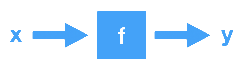
In mathematics, functions are mathematical equations, like \(f(x) = 2x^2\), that describe what you do to \(x\) to get \(y\) using mathematical operations. An R function that performs the same mathematical operations as \(f\) looks like this:

f <- function(x) {
  return(2*x^2)
}

Note the return at the end which signifies that the function f should have an explicit output. Not all code functions need to have an explicit output. Also, the return is technically not necessary. Whatever is on the last line of the function will automatically get returned as output. Let’s evaluate the R function f with different inputs. Guess the value before calling the function based on the equivalent mathematical function \(f(x) = 2x^2\). Feel free to change the input values!

Similar to mathematical functions, R functions expect a certain type of input. Make sure you know what data type the input should be in order for the function to work. Does our function f work for Boolean data types, for example?

Now try it out! Evaluate f with input TRUE and FALSE.

This works because R will coerce Boolean values to numerical values when in an arithmetical statement.

Question

What do you think will happen if I call f on an input vector, like f(c(2, 4))?

Many R functions that work on single numbers will also work on vectors by performing the function element-wise on each element of the vector.

Try and evaluate the function f on different vectors.

In general, an R function may have multiple inputs (called arguments) and only one output.

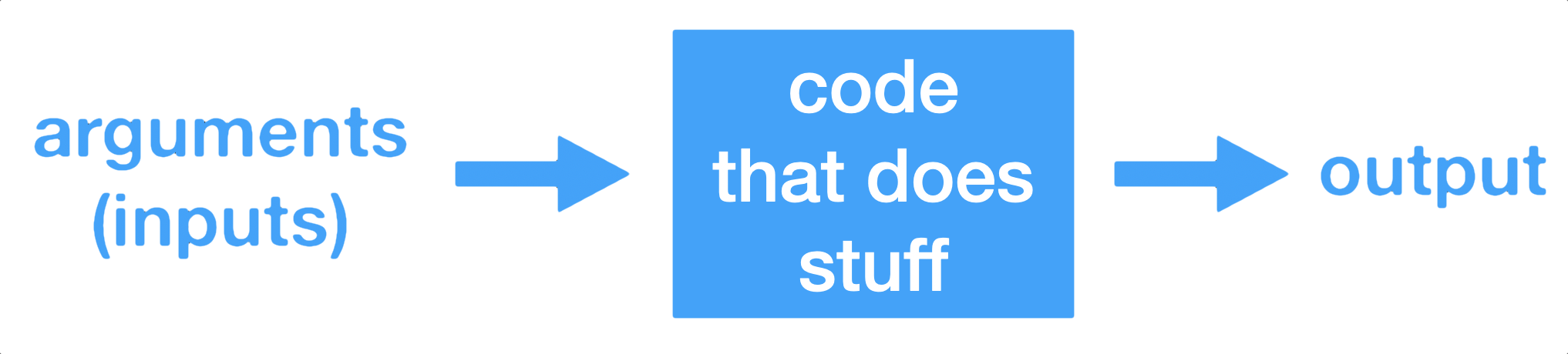
Besides being able to create our own function in R, it is important to learn how to use the plethora of existing R functions available to you. That is the subject of the next section.

Function documentation

Before even thinking of using an R function, you should clarify which arguments it expects. All the relevant details such as a description, usage, and arguments can be found in the documentation. To consult the documentation on the sd() function, for example, you can use one of following R commands:

help(sd)
?sd

Try one of these commands yourself in the console below to see what happens.

Another much more direct way to see just the arguments of the sd() function is the args() function. Try it out in the console:

Note the difference between the first argument x and the last argument na.rm. The last argument has a default value, meaning that you do not have to specify that argument in your call to the function. If you don’t specify it, the default will be used (e.g. na.rm is FALSE by default, which means don’t remove missing values by default). Since the first argument x does not have a default value, it is required - if you don’t give it a value, the function will likely not work.

So how do you specify function arguments when there are more than one? You can refer to function arguments by position and by name.

values <- c(1, 5, 6, 7)
sd(values)     # Specify by position

[1] 2.629956

sd(x = values) # Specify by name

[1] 2.629956

You can even do a combination of both. To illustrate this, let’s look at an example that has an NA (“not a number”) in one of the values. The value NA is useful to represent a missing value in your data.

values <- c(1, 5, 6, NA)
sd(values)

[1] NA

Note what happens by default when there is a missing value - sd returns NA! This is important to alert the data scientist that there might be missing values in your data. If you decide that omitting missing values in your calculation of the standard deviation is okay, then you can specify the second argument na.rm and set it to TRUE. Here are multiple ways to do that.

sd(values, TRUE)             # Specify both arguments by position
sd(values, na.rm = TRUE)     # Specify na.rm by name
sd(x = values, na.rm = TRUE) # Specify both by name
sd(na.rm = TRUE, x = values) # Specify both by name, but reversed order

The last command shows that named arguments can be specified in any order, as long as the ones specified by position are in the correct position. In this case, none were specified by position so we could put them in any order we wanted!

In the next exercises, you’ll be learning how to use the mean() function with increasing complexity. The first thing you’ll have to do is get acquainted with the mean() function.

Exercise 1: Consult the documentation on the mean() function

Consult the documentation on the mean() function: ?mean or help(mean).

Exercise 2: Inspect the arguments of the mean() function

Inspect the arguments of the mean() function using the args() function.

Solution

args(mean)

Use a function

The documentation on the mean() function gives us quite some information:

The mean() function computes the arithmetic mean.
The most general method takes multiple arguments: x and ....
The x argument should be a vector containing numeric, logical or time-related information.

Remember that R can match arguments both by position and by name. Can you still remember the difference? You’ll find out in this exercise!

Once more, you’ll be working with the view counts of your social network profiles for the past 7 days. These are stored in the linkedin and facebook vectors and have already been defined in the editor below.

linkedin <- c(16, 9, 13, 5, 2, 17, 14)
facebook <- c(17, 7, 5, 16, 8, 13, 14)

Exercise 1: Calculate average number of views

Calculate the average number of views for both linkedin and facebook and assign the result to avg_li and avg_fb, respectively. Experiment with different types of argument matching!

Solution

avg_li <- mean(linkedin)
avg_fb <- mean(facebook)

Exercise 2: Print average number of views

Print out both avg_li and avg_fb.

Solution

avg_li
avg_fb

Use a function: Optional arguments

Check the documentation on the mean() function again, paying particular attention to the Usage section:

The Usage section of the documentation includes two versions of the mean() function. The first usage,

mean(x, ...)

is the most general usage of the mean function. The ‘Default S3 method’, however, is:

mean(x, trim = 0, na.rm = FALSE, ...)

The ... is called dot-dot-dot, or ellipsis. It is a way for R to pass arguments along without the function having to name them explicitly.

For the next exercise, just work with the second usage of the mean function. Notice that both trim and na.rm have default values. Again, this makes them optional arguments.

Exercise 1: Calculate the mean of the sum

Calculate the mean of the element-wise sum of linkedin and facebook and assign the result to avg_sum.

Solution

avg_sum <- mean(linkedin + facebook)

Exercise 2: Calculate the trimmed mean of the sum

Calculate the mean once more, but this time set the trim argument equal to 0.2 and assign the result to avg_sum_trimmed.

Solution

avg_sum_trimmed <- mean(linkedin + facebook, trim = 0.2)

Exercise 3: Inspect both new variables

Print out both avg_sum and avg_sum_trimmed; can you spot the difference?

Solution

avg_sum
avg_sum_trimmed

Use a function: Missing values

Previously, we guided you through the example of specifying arguments of the sd() function. The sd() function has an optional argument, na.rm that specified whether or not to remove missing values from the input vector before calculating the standard deviation.

If you’ve had a good look at the documentation, you’ll know by now that the mean() function also has this argument, na.rm, and it does the exact same thing. By default, it is set to FALSE, as the Usage of the Default S3 method shows:

mean(x, trim = 0, na.rm = FALSE, ...)

Let’s see what happens if your vectors linkedin and facebook contain missing values (NA). Here are the previous linkedin and facebook vectors, now with some missing values inserted.

linkedin <- c(16, 9, 13, 5, NA, 17, 14)
facebook <- c(17, NA, 5, 16, 8, 13, 14)

Exercise 1: Basic average of linkedin

Calculate the average number of LinkedIn profile views, without specifying any optional arguments. Simply print the result to the console.

Solution

mean(linkedin)

Exercise 2: Advanced average of linkedin

Calculate the average number of LinkedIn profile views, but this time tell R to strip missing values from the input vector.

Solution

mean(linkedin, na.rm = TRUE)

Functions inside functions

You might remember that you can compose mathematical functions, where the output of one function is the input of another. If you have a function \(y = f(x)\) and another function \(z = g(y)\), then you can talk about the composite function \((g \circ f)(x) = g(f(x))\).

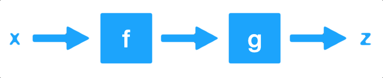
You can also compose functions in R using a similar syntax by embedding one function inside another.

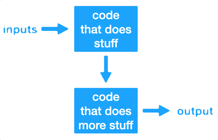
Here’s an example of composing the functions paste() and print() that you’ve seen in a previous exercise:

speed <- 31
print(paste("Your speed is", speed))

[1] "Your speed is 31"

Notice that both the print() and paste() functions use the ellipsis - ... - as an argument. Can you figure out how they’re used?

For the next exercise, we’ll start again with the linkedin and facebook vectors that contain missing values.

linkedin <- c(16, 9, 13, 5, NA, 17, 14)
facebook <- c(17, NA, 5, 16, 8, 13, 14)

Exercise 1: Calculate the mean absolute deviation

Use abs() on linkedin - facebook to get the absolute differences between the daily Linkedin and Facebook profile views. Next, use this function call inside mean() to calculate the Mean Absolute Deviation. In the mean() call, make sure to specify na.rm to treat missing values correctly!

Solution

mean(abs(linkedin - facebook), na.rm = TRUE)

Required, or optional?

By now, you will probably have a good understanding of the difference between required and optional arguments. Let’s refresh this difference by having one last look at the mean() function:

mean(x, trim = 0, na.rm = FALSE, ...)

x is required; if you do not specify it, R will throw an error. trim and na.rm are optional arguments: they have a default value which is used if the arguments are not explicitly specified.

Check the arguments for the read.table() function in the following console to answer the next question.

Question

“Which of the following statements about the read.table() function are true?”

Using functions that are already available in R is pretty straightforward, but how about writing your own functions to supercharge your R programs?

Write your own function

Wow, things are getting serious… You’re about to write your own function! You already saw a function f that was created in the beginning of this chapter to perform computationally the same operations as the mathematical function \(f(x) = 2x^2\). Before you have a go at creating your own function, have a look at the following function template:

my_fun <- function(arg1, arg2) {
  body
}

Notice that this recipe uses the assignment operator (<-) just as if you were assigning a vector to a variable for example. This is not a coincidence. Creating a function in R basically is the assignment of a function object to a variable! In the recipe above, you’re creating a new R variable my_fun, that becomes available in the workspace as soon as you execute the definition. From then on, you can use the my_fun as a function.

Exercise 1: Create a function pow_two()

Create a function pow_two(): it takes one argument x and returns that number squared (that number times itself).

Solution

pow_two <- function(x) {
  x * x
}

Exercise 2: Use the function

Call this newly defined function with 12 as input.

Solution

pow_two(12)

Exercise 3: Create a function sum_abs()

Next, create a function sum_abs(), that takes two arguments a and b and returns the sum of the absolute values of both arguments.

Solution

sum_abs <- function(a, b) {
  abs(a) + abs(b)  
}

Exercise 4: Use the function

Finally, call the function sum_abs() with arguments -2 and 3 afterwards.

Solution

sum_abs(-2, 3)

Write your own function: No arguments

There are situations in which your function does not require an input. Let’s say you want to write a function that gives us the random outcome of throwing a fair die:

throw_die <- function() {
  number <- sample(1:6, size = 1)
  number
}

throw_die()

[1] 3

In the next exercise, you will code a function that doesn’t take any arguments!

Exercise 1: Define the function hello()

Define a function, hello(). It prints out “Hi there!” and returns TRUE. It has no arguments.

Solution

hello <- function() {
  print("Hi there!")
  return(TRUE)
}

Exercise 2: Call the function hello()

Call the function hello(), without specifying arguments of course.

Solution

hello()

Write your own function: Default values

Do you still remember the difference between an argument with and without default values? Have another look at the sd() function by typing ?sd in the console. The usage section shows the following information:

sd(x, na.rm = FALSE)

This tells us that x has to be defined for the sd() function to be called correctly. However, na.rm already has a default value and not specifying this argument won’t cause an error.

You can define default argument values in your own R functions as well. You can use the following recipe to do so:

my_fun <- function(arg1, arg2 = val2) {
  body
}

Exercise: Finish the pow_two() function

The editor below contains an extended version of the pow_two() function from before. Can you finish it?

Add an optional argument, named print_info, that is TRUE by default.
Wrap an if construct around the print() function: this function should only be executed if print_info is TRUE.
Feel free to experiment with the pow_two() function you’ve just coded.

Solution

pow_two <- function(x, print_info = TRUE) {
  y <- x * x
  if (print_info == TRUE){
    print(paste(x, "to the power two equals", y))
  }
  return(y)
}

Function scoping

An issue that we have not discussed yet is function scoping. It implies that variables that are defined inside a function are not accessible outside that function. Try running the following code and see if you understand the results:

y was defined inside the pow_two() function and therefore it is not accessible outside of that function. This is also true for the function’s arguments of course - x in this case.

Question

Consider the following chunk of code:

Which statement is correct about the function two_dice()? Feel free to check each option in the code editor above if you are unsure.

If you’re familiar with other programming languages, you might wonder whether R passes arguments by value or by reference. Find out in the next exercise!

R passes arguments by value

The title gives it away already: R passes arguments by value. What does this mean? Simply put, it means that an R function cannot change the variable that you input to that function. Let’s look at a simple example (try it in the editor):

Inside the triple() function, the argument x gets overwritten with its value times three. Afterwards this new x is returned. If you call this function with a variable a set equal to 5, you obtain 15. But did the value of a change? If R were to pass a to triple() by reference, the override of the x inside the function would ripple through to the variable a, outside the function. However, R passes by value, so the R objects you pass to a function can never change unless you do an explicit assignment. a remains equal to 5, even after calling triple(a). Basically, you can think of R as making a copy of the value of a and assigning it to the argument x.

Question

Consider the following chunk of code:

increment <- function(x, inc = 1) {
  x <- x + inc
  x
}
    
count <- 5
a <- increment(count, 2)
b <- increment(count)
count <- increment(count, 2)

Can you tell which one of the following statements is false about the above piece of code?

Given that R passes arguments by value and not by reference, the value of count is not changed after the first two calls of increment(). Only in the final expression, where count is re-assigned explicitly, does the value of count change.

R you functional?

Now that you’ve acquired some skills in defining functions with different types of arguments and return values, you should try to create more advanced functions. As you’ve noticed in the previous exercises, it’s perfectly possible to add control-flow constructs, loops and even other functions to your function body.

Remember our social media example? The vectors linkedin and facebook are already defined in the workspace so you can get your hands dirty straight away. As a first step, you will be writing a function that can interpret a single value of this vector. In the next exercise, you will write another function that can handle an entire vector at once.

linkedin <- c(16, 9, 13, 5, 2, 17, 14)
facebook <- c(17, 7, 5, 16, 8, 13, 14)

Exercise: Define the interpret function

Finish the function definition for interpret(), that interprets the number of profile views on a single day:
The function takes one argument, num_views.
If num_views is greater than 15, the function prints out “You’re popular!” to the console and returns num_views.
Else, the function prints out “Try to be more visible!” and returns 0.
Finally, call the interpret() function twice: on the first value of the linkedin vector and on the second element of the facebook vector.

Solution

interpret <- function(num_views) {
  if (num_views > 15) {
    print("You're popular!")
    return(num_views)
  } else {
    print("Try to be more visible!")
    return(0)
  }
}

# Call the interpret function twice
interpret(linkedin[1])
interpret(facebook[2])

R you functional? Inception-style!

A possible implementation of the interpret() function is already available in the editor. In this exercise you’ll be writing another function that will use the interpret() function to interpret all the data from your daily profile views inside a vector. Furthermore, your function will return the sum of views on popular days, if asked for. A for loop is ideal for iterating over all the vector elements. The ability to return the sum of views on popular days is something you can code through a function argument with a default value.

As before, the linkedin and facebook vectors are available to you.

linkedin <- c(16, 9, 13, 5, 2, 17, 14)
facebook <- c(17, 7, 5, 16, 8, 13, 14)

Exercise 1: Define the interpret_all() function

Finish the template for the interpret_all() function:

Make return_sum an optional argument, that is TRUE by default.
Inside the for loop, iterate over all views: on every iteration, add the result of interpret(v) to count. Remember that interpret(v) returns v for popular days, and 0 otherwise. At the same time, interpret(v) will also do some printouts.
Create an if construct so that if return_sum is TRUE, return count and else, return NULL.

Call this newly defined function on both linkedin and facebook.

Solution

interpret <- function(num_views) {
  if (num_views > 15) {
    print("You're popular!")
    return(num_views)
  } else {
    print("Try to be more visible!")
    return(0)
  }
}

# Define the interpret_all() function
# views: vector with data to interpret
# return_sum: return total number of views on popular days?
interpret_all <- function(views, return_sum = TRUE) {
  count <- 0

  for (v in views) {
    count <- count + interpret(v)
  }

  # Insert if-else statement on the next line
  if (return_sum == TRUE) {
    return(count)
  } else {
    return(NULL)
  }
}

# Call the interpret_all() function on both linkedin and facebook
interpret_all(linkedin)
interpret_all(facebook)

Are R functions black boxes?

Sometimes functions can be referred to as “black boxes” when you use them but are unable to see their code. A very useful thing to know in R is that for many functions you can easily see their code by calling the print function with the function name of interest. For example:

print(sd)

function (x, na.rm = FALSE) 
sqrt(var(if (is.vector(x) || is.factor(x)) x else as.double(x), 
    na.rm = na.rm))
<bytecode: 0x7fe15842a578>
<environment: namespace:stats>

Try it now!

Exercise: Peeking into function code

The interpret and interpret_all functions from the previous exercise are loaded in memory. Use the print command to show their code!

Functions really are variables!

To drive home the point that functions really are variables (i.e. they are variables with data type “function”), we will revisit a rather embarrassing point in American history known as the Indiana Pi Bill. Here’s how the Wikipedia article describes it:

The Indiana Pi Bill is the popular name for bill #246 of the 1897 sitting of the Indiana General Assembly, one of the most notorious attempts to establish mathematical truth by legislative fiat.

The legislation had the title “A Bill for an act introducing a new mathematical truth and offered as a contribution to education to be used only by the State of Indiana free of cost by paying any royalties whatever on the same, provided it is accepted and adopted by the official action of the Legislature of 1897.” In any case, the bill (and the mathematical “alternative facts” that it contained) implied that the value of \(\pi\) was 3.2.

Suppose we had the following extremely simple function inspired by this lovely story. Rather than using 3.2 for \(\pi\), we’ll round to the nearest hundredth using the very useful signif function.

indiana_pi <- function() {
  return(signif(pi, digits=3))
}

Rather than re-code the function, let’s rename it to something more appropriate.

Exercise: A round pi

The function indiana_pi is already available in your workspace. Assign the function to a new variable named round_to_hundredth and run the function to make sure it “works”.

Solution

round_to_hundredth <- indiana_pi
round_to_hundredth()

Leci n’est pas une pipe

The Treachery of Images is a painting by surrealist painter René Magritte. It was the inspiration (at least in name and design) for one of the most helpful functions/operators in R for data science called the pipe operator and denoted %>%. This operator is included in the R package magrittr, which has the following awesome hex sticker for its package.

This operator was so successful that R created its own pipe operator (|>), so the additional magrittr package would not be necessary.

The inspiration for a pipe operator comes about when thinking about how much data processing must be done with data: import data, clean data, rename variables, filter observations, select variables, calculate statistics, … If each one of these steps is an R function, where the output of one step becomes the input of another, your code can become quickly unreadable as an onion of function calls, with layer-upon-layer of parenthetical embedded statements.

Here’s an example using some functions in the tidyverse that we’ll learn more about later. It loads in data, selects certain variables, filters (subsets) the result based on a condition, specifies a grouping categorical variables to compute a statistic over, and finally computes the average of a numerical variable over these specified groups. Note that the last two steps (group_by and summarize) perform similar operations as the tapply operation that you’ve used before. Here’s the code:

library(tidyverse)

summarize(group_by(filter(select(read_csv("data/chap03q14VasopressinVoles.csv"), c(treatment, percent)), percent >= 50), treatment), mean(percent))

# A tibble: 2 × 2
  treatment `mean(percent)`
  <chr>               <dbl>
1 control              75.8
2 enhanced             86.3

What the heck is going on?!?! What a mess. The situation can be improved a bit by some proper formatting of the code (remember, indentations and new lines are your friends - let your code breathe!)

library(tidyverse)

summarize(
  group_by(
    filter(
      select(
        read_csv("data/chap03q14VasopressinVoles.csv"), 
        c(treatment, percent)), 
      percent >= 50), 
    treatment), 
  mean(percent)
)

That’s a little better. We can more easily see the functions that are being called, but it’s still hard to see which arguments go with which function (percent >= 50 goes with select or filter?) Indentation helps, but still difficult to read. Also, to see the proper order that the functions are called, you have to start in the inside of the “onion” and work your way out. Very confusing! What if we had an operator that matched more our “function box” image?

We do! That’s exactly what the pipe operator |> gives us. In the image above, replace the arrows with the pipe operator. The image of a pipe illustrates that data flows through the functions as input and comes out as output. Here’s the same code from above, but now we use the pipe operator.

read_csv("data/chap03q14VasopressinVoles.csv") |>
  select(c(treatment, percent)) |>
  filter(percent >= 50) |>
  group_by(treatment) |>
  summarize(mean(percent))

# A tibble: 2 × 2
  treatment `mean(percent)`
  <chr>               <dbl>
1 control              75.8
2 enhanced             86.3

So much easier! Now you can actually read the code from left-to-right (or top-to-bottom), and the function arguments are exactly with the function they belong to.

“But wait!”, some of you might be saying. “If a function has multiple arguments, how does the pipe operator know which argument to assign the input on the left to??” Great question! The pipe operator will assign the left object (the input) to the first argument of the function on the right of the pipe. As an example, the following two statements are equivalent:

# This command without the pipe...
filter(mydata, percent >= 50)

# ...is equivalent to this one with the pipe...
mydata |> filter(percent >= 50)

For the following exercise, we will consider Exercise 32 in Chapter 2 of Whitlock & Schluter’s textbook “The Analysis of Biological Data”.

More than 10% of people carry the parasite Toxoplasma gondhii. The following table gives data from Prague on 15- to 29-year old drivers who had been involved in an accident. The table gives the number of drivers who were infected with Toxoplasma gondhii and who were uninfected. These numbers are compared with a control sample of 249 drivers of the same age living in the same area who had not been in an accident.

           infectionStatus
driverType  infected uninfected
  accidents       21         38
  control         38        211

Exercise 1: I love mosaic plots!

First, use read.csv to load in the data located at data/chap02q32ToxoplasmaAccidents.csv and store in the variable toxoData.
Next, use the table command to recreate the table above and store the result in the variable toxoTable.
Finally, use the mosaicplot command with toxoTable as the argument to create a mosaic plot.

Solution

toxoData <- read.csv("data/chap02q32ToxoplasmaAccidents.csv")
toxoTable <- table(toxoData)
mosaicplot(toxoTable)

Exercise 2: I love mosaic plots with pipes!

Use the pipe operator below to perform the same operations as Exercise 1.

Solution

read.csv("data/chap02q32ToxoplasmaAccidents.csv") |>
  table() |>
  mosaicplot()

Congratulations! You have finished Chapter 3!

You have finished the chapter “Functions”!

Chap. 1: Conditionals and control flow

Equality and inequality

Data type: Boolean

Data type: String

Data type: Numeric

Greater and less than

Compare vectors

Compare matrices

Logical Operators: AND (&), OR (|) and NOT (!)

Logical Operators: Vectorized!

Reverse the result: !

Blend it all together

Conditional statements: The if statement

Add an else

Customize further: else if

Else if 2.0

Take control!

Congratulations! You’ve finished Chapter 1!

Chap. 2: Loops

Write a while loop

Throw in more conditionals

Stop the while loop with break

Build a while loop from scratch

For loops

Looping over a vector

Looping over a list

Breaking out of a for loop

Skipping values in a for loop

For loops (version 2): Looping with indices instead of values

Wrap-up: for loops

Loop over a list

Loop over a matrix

Mix it up with control flow

Next, you break it

Build a for loop from scratch

Congratulations! You’ve finished Chapter 2!

Chap. 3: Functions

Definitions

Function documentation

Use a function

Use a function: Optional arguments

Use a function: Missing values

Functions inside functions

Required, or optional?

Write your own function

Write your own function: No arguments

Write your own function: Default values

Function scoping

R passes arguments by value

R you functional?

R you functional? Inception-style!

Are R functions black boxes?

Functions really are variables!

Leci n’est pas une pipe

Congratulations! You have finished Chapter 3!

Logical Operators: AND (`&`), OR (`|`) and NOT (`!`)

Wrap-up: `for` loops